I wrote this article for two target audiences: first, for those who want to learn about the steps involved in calculating the lens, and second, for anyone interested in the history and qualitative classification of the Minostigmat.
Click here to go directly to the calculation.
A Trip to Riga and Its Consequences
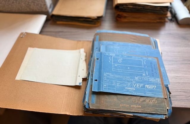
When my friend Burkhard, also a Minox Riga enthusiast, traveled to Riga this summer, tracking down the VEF Minox was at the top of his list. At my request, he also searched for the design drawings for this camera’s lens, the Minostigmat. I intended to use it for a Minox lens calculation.
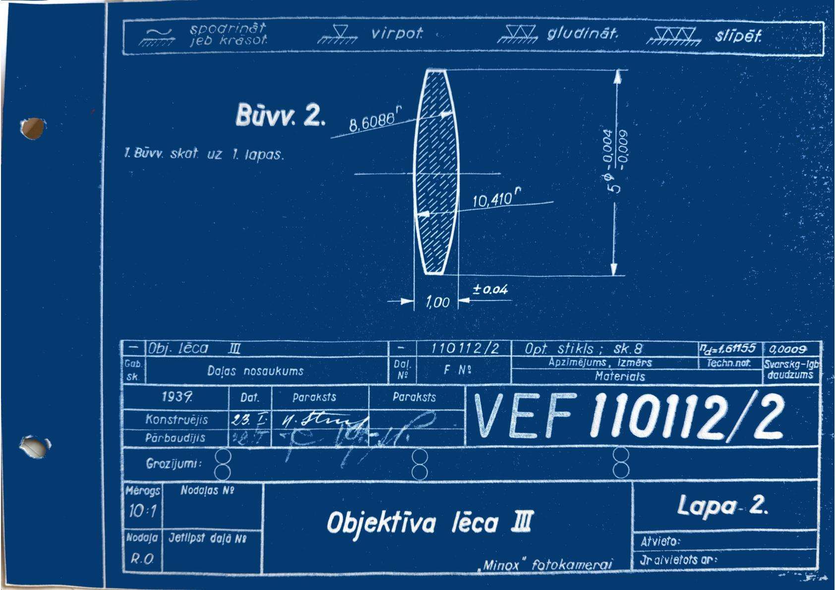
And he found what he was looking for at the VEF History Museum. With the help of Dace Kaprāne, the chief curator, he located them in the archives. Tucked away in a folder, he actually found what I had been looking for for a long time but couldn’t find anywhere: the original drawings of the Minostigmat.
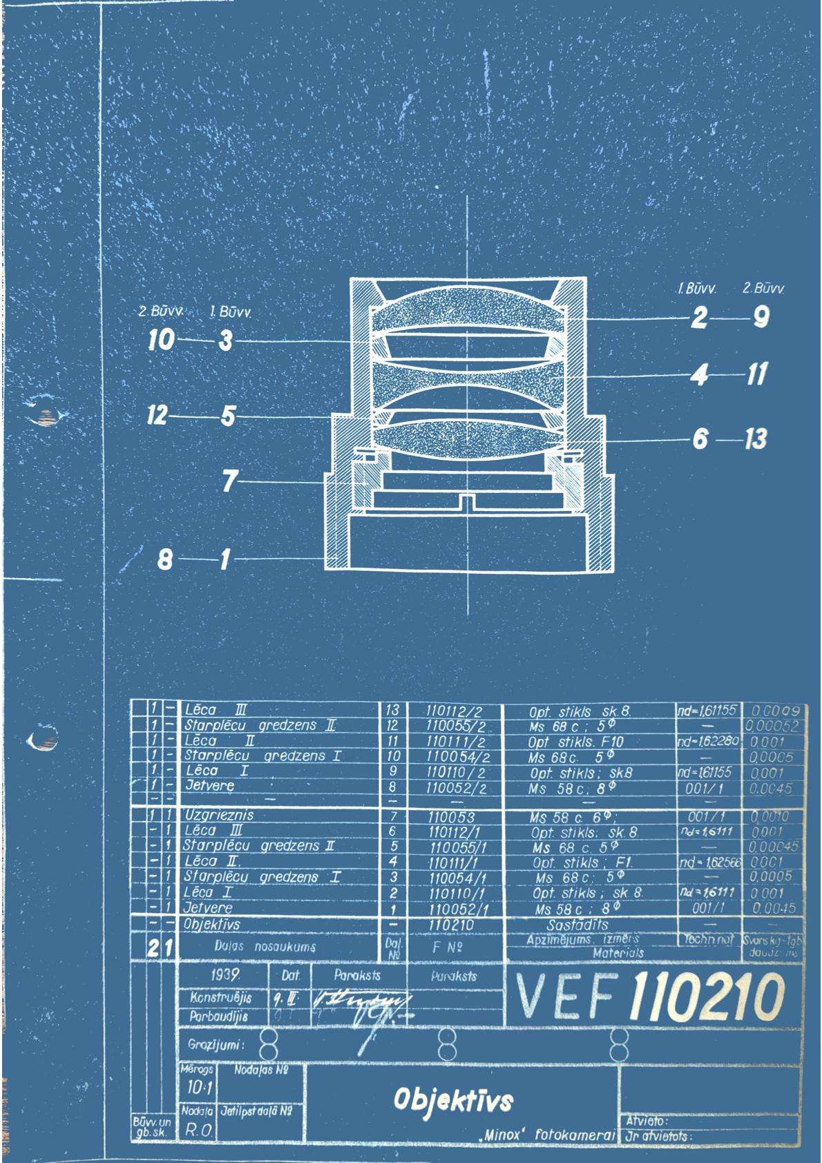
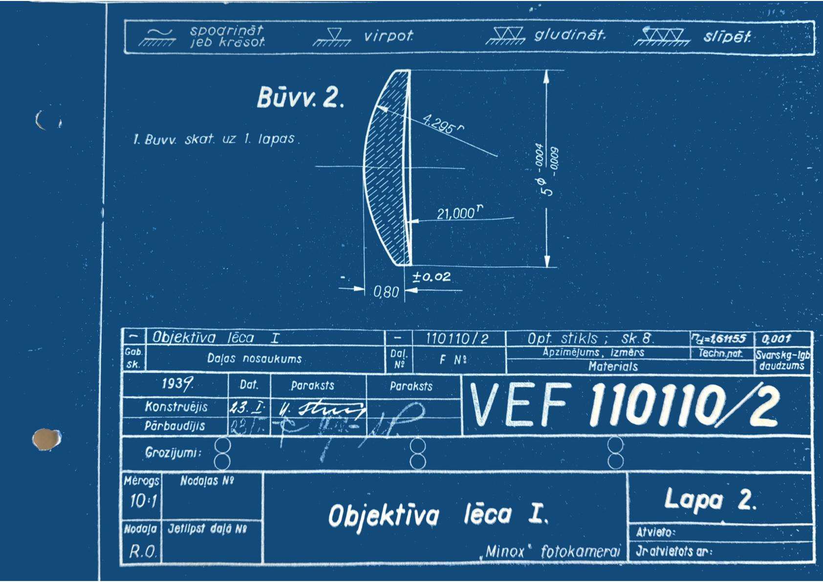
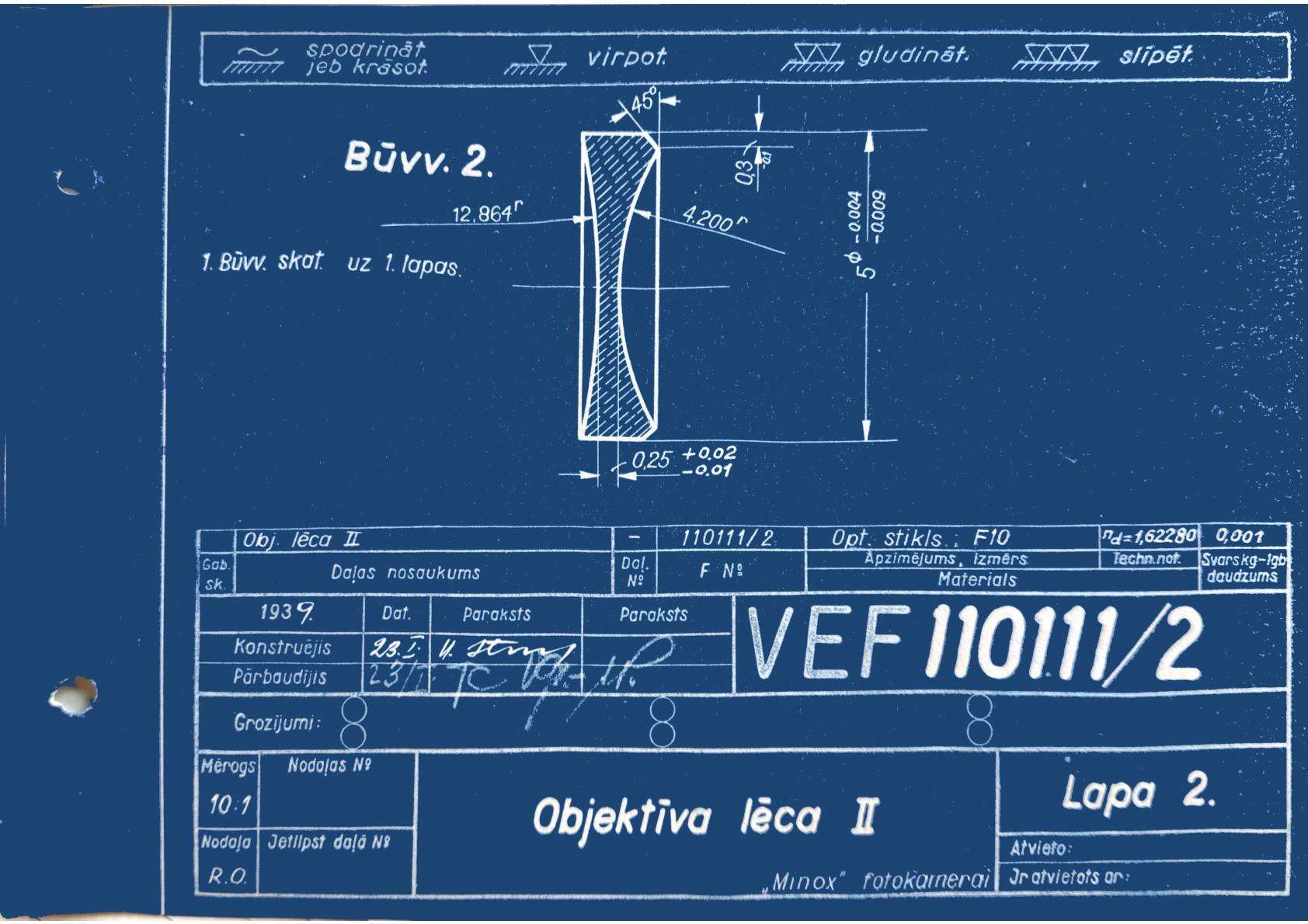
So here, courtesy of the VEF History Museum, are the blueprints for the manufacture of the famous lens, published for the first time:
Expectations, theory, and reality
I had been searching for the exact specifications of the Minostigmat for quite some time because I was determined to calculate its imaging performance. After measuring its performance in practice in 2024, I wanted to compare the two sets of results. I was also interested in the optical parameters so that I could evaluate this lens in general.
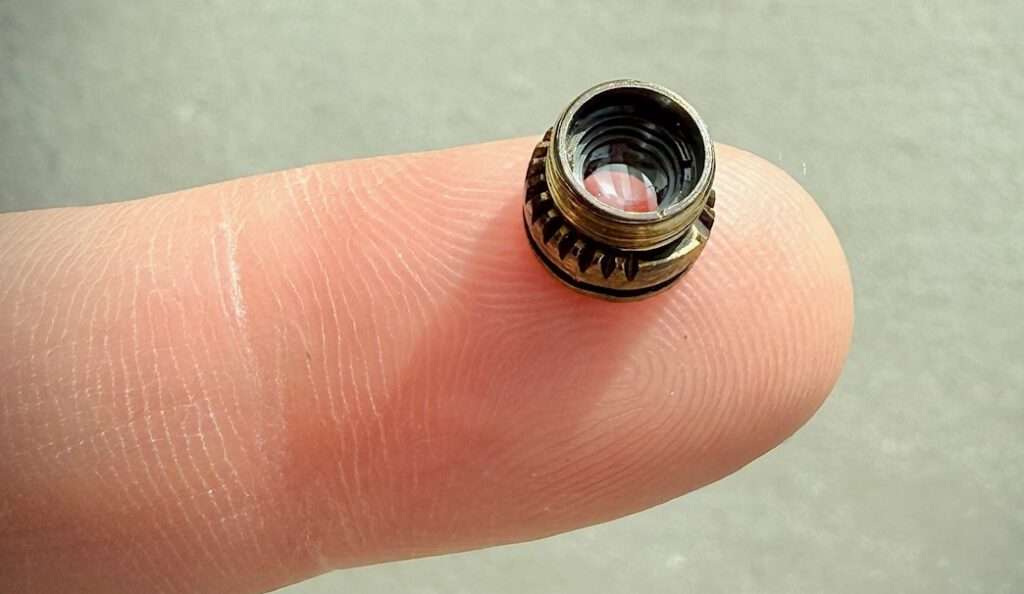
The results I’m about to present here are impressive in two respects. First of all, the specifications show just how outstanding this lens is, even in theory. On top of that, there’s the astonishingly good correlation with my earlier practical measurements using test charts.
You can find a brief, easy-to-understand introduction to how a design engineer goes about designing a Cooke triplet here.
So that you can follow along with the calculations below on your own, I’ve broken everything down into the smallest possible steps using specific numbers. This way, you can verify all the results yourself using a calculator. While this makes the article a bit long, it ensures that everything is transparent.
Join me on this exciting journey through the process of calculating a lens. Don’t worry – the four basic arithmetic operations are all you need.
If you’re not interested in the calculations, you can go directly to the results.
What is the purpose of lens calculation?
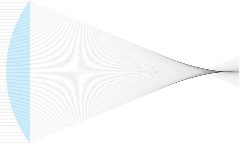
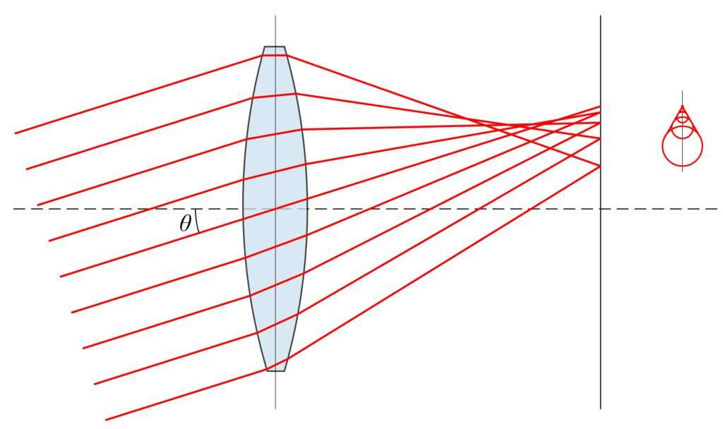
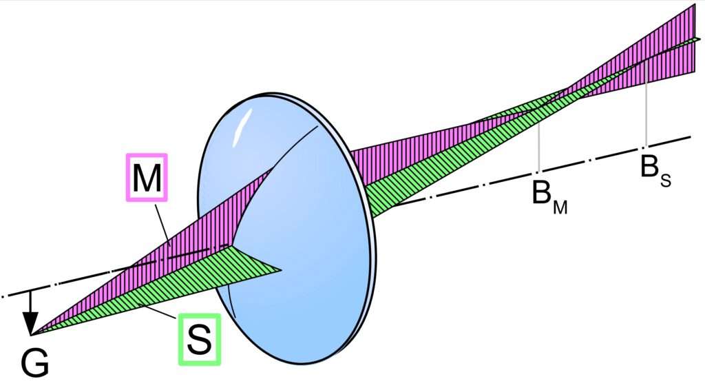
In optics, aberrations are defined as deviations from the ideal optical image produced by an optical system. All of the monochromatic aberrations (Spherical aberration, Coma, Astigmatism, Field curvature, Image distortion) considered here overlap, and any change in the optical system affects all aberrations in a generally nonlinear manner.
To evaluate the quality of a lens design, it is necessary to know the magnitude of the aberrations in total. To calculate this , the German scientist Philipp Ludwig von Seidel developed a mathematical method in 1857. He arrived at the following equation, which calculates the total aberration, the wavefront deviation:
W(h, ρ, θ) = ⅛·S_I·ρ⁴ + ½·S_II·h·ρ³·cosθ + ½·S_III·h²·ρ²·cos²θ + ¼·(S_III + S_IV)·h²·ρ² + ½·S_V·h³·ρ·cosθ
Don’t worry, we won’t have to calculate the formula above ourselves. Instead, I’ve turned it into a chart, which I’ll present along with the results.
Explanation of the variables:
- W: Wavefront deviation. Describes the magnitude of the total aberration.
- h: Field height (0…1). Describes where the point being viewed is located within the image area. A point at, for example, h = 0.7 would lie at 70% of the distance from the center to the corner.
- ρ: normalized pupil radius (0…1). Describes which part of the entrance pupil (aperture) the observed ray passes through—measured radially. For the Minostigmat, ρ = 1 corresponds to a ray at y = 2.142857 mm (half the lens diameter).
- θ: Azimuth angle in the pupil (0…360°). Describes the angular position within the pupil, not within the field of view.
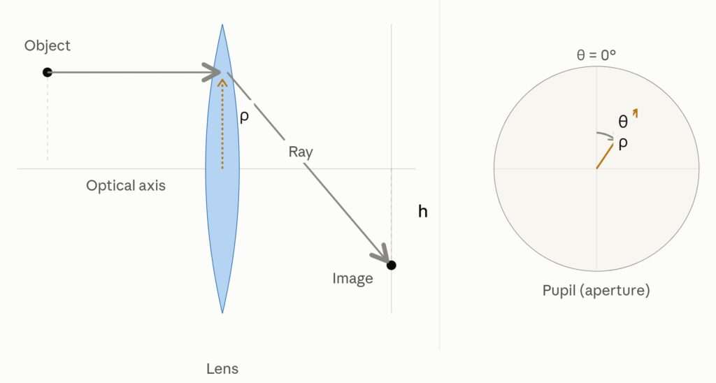
- S_I, S_II, S_III, S_IV, S_V: These are the so-called Seidel coefficients. They are calculated for the five types of aberrations based on the lens design data. This is the main computational work.
Once we have calculated these five coefficients for the minostigmat, we can determine the aberration for every point in the image.
Focal length
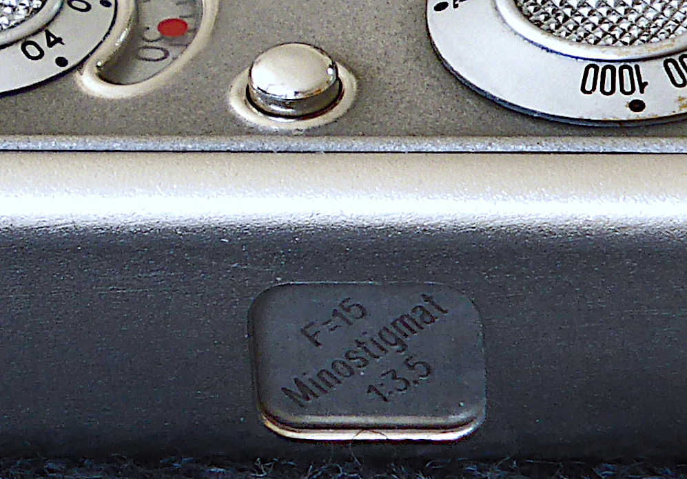
My first step was to verify the plausibility of the Minostigmat drawings and the values derived from them. A good way to do this is to calculate the focal length based on this information. The result is known: it should be 15 mm.
However, there was another problem. As you can see in the assembly drawing above, the two dimensions for the distances between the three lenses are missing. I therefore had to measure these dimensions directly from the drawing. Of course, this is subject to reading errors. Both dimensions (d2 and d4, see picture below) strongly influence the calculation of the focal length. Using my measured values, the focal length comes out to 14.73 mm. This is close to the expected value.
However, it’s safe to assume that d2 and d4 were chosen so that the focal length is exactly 15 mm. I therefore varied these two values over several iterations so that the deviation from my measured values is minimal and a focal length of 15 mm is obtained.
As a result, the value I measured for d2 changes from 1.25 mm to 1.1265 mm, and the value for d4 changes from 1.10 mm to 0.9520 mm. I then performed all calculations using these values.
The Matrix Method
It is worth noting that the elegant 2×2 matrix formalism, which is now standard in optical design, did not yet exist when Hans Schulz calculated the Minostigmat in 1935. Each refracting surface and each air gap is represented by a small matrix, and the entire system reduces to a single matrix product. The explicit matrix method for lens design was first formalized fifteen years later, in Clyde W. Harris’s 1950 paper “Optical Design by a Matrix Method”, which showed how interval and surface matrices could be multiplied together to yield the paraxial, aberrational, and even chromatic behavior of a complete system in a single, compact operation. I will use this method in the following.
In the calculations, I use the symbols according to standard convention:
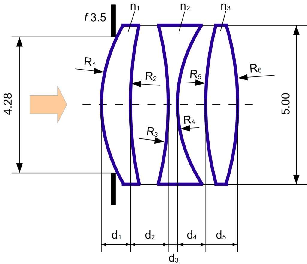
I took the specific dimensions and the refractive indices n from the VEF drawings from 1939 shown above. The following two tables show the numerical values.
Calculation of the focal length
First, we compile all the data we can derive from the drawings. This includes the radii, thicknesses, refractive indices, and distances between the three lenses.
We organize this information according to the matrix method’s system, listing the six surfaces of the three lenses from left to right. For each surface, we specify the refractive index (before) on the left and right sides (after) of the lens.
We also sort the distances and thicknesses of the lenses from left to right.
Click to expand: Input data
0. Input Data
| Surface | R (mm) | n (before) | n’ (after) |
|---|---|---|---|
| 1 | 4.2950 | 1.0000 (air) | 1.6116 |
| 2 | 21.0000 | 1.6116 | 1.0000 (air) |
| 3 | -12.8640 | 1.0000 (air) | 1.6228 |
| 4 | 4.2000 | 1.6228 | 1.0000 (air) |
| 5 | 10.4100 | 1.0000 (air) | 1.6116 |
| 6 | -8.6086 | 1.6116 | 1.0000 (air) |
| Gap | d (mm) | n |
|---|---|---|
| d1 (inside lens 1) | 0.800000 | 1.6116 |
| d2 (air, 1→2) | 1.126477 (measured: 1.25) | 1.0000 |
| d3 (inside lens 2) | 0.250000 | 1.6228 |
| d4 (air, 2→3) | 0.952009 (measured: 1.10) | 1.0000 |
| d5 (inside lens 3) | 1.000000 | 1.6116 |
1. Refraction Matrices R1–R6
Formula: \(C = -\dfrac{n’-n}{R\cdot n’}\), \(D=\dfrac{n}{n’}\)
$$R_1 = \begin{pmatrix} 1 & 0 \\ -0.088358 & 0.620501 \end{pmatrix}$$
$$R_2 = \begin{pmatrix} 1 & 0 \\ 0.029124 & 1.611600 \end{pmatrix}$$
$$R_3 = \begin{pmatrix} 1 & 0 \\ 0.029834 & 0.616219 \end{pmatrix}$$
$$R_4 = \begin{pmatrix} 1 & 0 \\ 0.148286 & 1.622800 \end{pmatrix}$$
$$R_5 = \begin{pmatrix} 1 & 0 \\ -0.036455 & 0.620501 \end{pmatrix}$$
$$R_6 = \begin{pmatrix} 1 & 0 \\ -0.071045 & 1.611600 \end{pmatrix}$$
2. Translation Matrices T1–T5
Note: The ray-transfer vector used here carries the real ray angle u (not the reduced angle n·u), so the translation matrix is \(T=\begin{pmatrix}1 & d\\0 & 1\end{pmatrix}\) — without dividing by n.
$$T=\begin{pmatrix}1 & d\\0 & 1\end{pmatrix} \quad \text{(no division by n)}$$
$$T_1 = \begin{pmatrix} 1 & 0.800000 \\ 0 & 1 \end{pmatrix}$$
$$T_2 = \begin{pmatrix} 1 & 1.126477 \\ 0 & 1 \end{pmatrix} \quad $$
$$T_3 = \begin{pmatrix} 1 & 0.250000 \\ 0 & 1 \end{pmatrix}$$
$$T_4 = \begin{pmatrix} 1 & 0.952009 \\ 0 & 1 \end{pmatrix} \quad $$
$$T_5 = \begin{pmatrix} 1 & 1.000000 \\ 0 & 1 \end{pmatrix}$$
3. Sequential Matrix Multiplication
$$M = R_6 \cdot T_5 \cdot R_5 \cdot T_4 \cdot R_4 \cdot T_3 \cdot R_3 \cdot T_2 \cdot R_2 \cdot T_1 \cdot R_1$$
Product rule for \(X=\begin{pmatrix}a&b\\c&d\end{pmatrix}\), \(P=\begin{pmatrix}e&f\\g&h\end{pmatrix}\):
$$X \cdot P = \begin{pmatrix} ae+bg & af+bh \\ ce+dg & cf+dh \end{pmatrix}$$
Click to expand: Step-by-step calculations with full numerical data
Each step below shows the multiplication in three lines: the two matrices being multiplied, then the elementwise arithmetic, then the numeric result — each continuation line starts
Start: P0 = R1$$P_0 = \begin{pmatrix} 1 & 0 \\ -0.088358 & 0.620501 \end{pmatrix}$$
Step 1: P1 = T1 · P0$$P_1 = \begin{pmatrix} 1 & 0.8 \\ 0 & 1 \end{pmatrix}\begin{pmatrix} 1 & 0 \\ -0.088358 & 0.620501 \end{pmatrix}$$
$$= \begin{pmatrix} 1\cdot1+0.8\cdot(-0.088358) & 1\cdot0+0.8\cdot0.620501 \\ 0\cdot1+1\cdot(-0.088358) & 0\cdot0+1\cdot0.620501 \end{pmatrix}$$
$$= \begin{pmatrix} 0.929314 & 0.496401 \\ -0.088358 & 0.620501 \end{pmatrix}$$
Step 2: P2 = R2 · P1$$P_2 = \begin{pmatrix} 1 & 0 \\ 0.029124 & 1.611600 \end{pmatrix}\begin{pmatrix} 0.929314 & 0.496401 \\ -0.088358 & 0.620501 \end{pmatrix}$$
$$= \begin{pmatrix} 1\cdot 0.929314+0\cdot(-0.088358) & 1\cdot 0.496401+0\cdot 0.620501 \\ 0.029124\cdot 0.929314+1.611600\cdot(-0.088358) & 0.029124\cdot 0.496401+1.611600\cdot 0.620501 \end{pmatrix}$$
$$= \begin{pmatrix} 0.929314 & 0.496401 \\ -0.115333 & 1.014459 \end{pmatrix}$$
Step 3: P3 = T2 · P2$$P_3 = \begin{pmatrix} 1 & 1.126477 \\ 0 & 1 \end{pmatrix}\begin{pmatrix} 0.929314 & 0.496401 \\ -0.115333 & 1.014459 \end{pmatrix}$$
$$= \begin{pmatrix} 1\cdot 0.929314+1.126477\cdot(-0.115333) & 1\cdot 0.496401+1.126477\cdot 1.014459 \\ 0\cdot 0.929314+1\cdot(-0.115333) & 0\cdot 0.496401+1\cdot 1.014459 \end{pmatrix}$$
$$= \begin{pmatrix} 0.799393 & 1.639162 \\ -0.115333 & 1.014459 \end{pmatrix}$$
Step 4: P4 = R3 · P3$$P_4 = \begin{pmatrix} 1 & 0 \\ 0.029834 & 0.616219 \end{pmatrix}\begin{pmatrix} 0.799393 & 1.639162 \\ -0.115333 & 1.014459 \end{pmatrix}$$
$$= \begin{pmatrix} 1\cdot 0.799393+0\cdot(-0.115333) & 1\cdot 1.639162+0\cdot 1.014459 \\ 0.029834\cdot 0.799393+0.616219\cdot(-0.115333) & 0.029834\cdot 1.639162+0.616219\cdot 1.014459 \end{pmatrix}$$
$$= \begin{pmatrix} 0.799393 & 1.639162 \\ -0.047236 & 0.674033 \end{pmatrix}$$
Step 5: P5 = T3 · P4$$P_5 = \begin{pmatrix} 1 & 0.25 \\ 0 & 1 \end{pmatrix}\begin{pmatrix} 0.799393 & 1.639162 \\ -0.047236 & 0.674033 \end{pmatrix}$$
$$= \begin{pmatrix} 1\cdot 0.799393+0.25\cdot(-0.047236) & 1\cdot 1.639162+0.25\cdot 0.674033 \\ 0\cdot 0.799393+1\cdot(-0.047236) & 0\cdot 1.639162+1\cdot 0.674033 \end{pmatrix}$$
$$= \begin{pmatrix} 0.787584 & 1.807670 \\ -0.047236 & 0.674033 \end{pmatrix}$$
Step 6: P6 = R4 · P5$$P_6 = \begin{pmatrix} 1 & 0 \\ 0.148286 & 1.622800 \end{pmatrix}\begin{pmatrix} 0.787584 & 1.807670 \\ -0.047236 & 0.674033 \end{pmatrix}$$
$$= \begin{pmatrix} 1\cdot 0.787584+0\cdot(-0.047236) & 1\cdot 1.807670+0\cdot 0.674033 \\ 0.148286\cdot 0.787584+1.622800\cdot(-0.047236) & 0.148286\cdot 1.807670+1.622800\cdot 0.674033 \end{pmatrix}$$
$$= \begin{pmatrix} 0.787584 & 1.807670 \\ 0.040137 & 1.361738 \end{pmatrix}$$
Step 7: P7 = T4 · P6$$P_7 = \begin{pmatrix} 1 & 0.952009 \\ 0 & 1 \end{pmatrix}\begin{pmatrix} 0.787584 & 1.807670 \\ 0.040137 & 1.361738 \end{pmatrix}$$
$$= \begin{pmatrix} 1\cdot 0.787584+0.952009\cdot 0.040137 & 1\cdot 1.807670+0.952009\cdot 1.361738 \\ 0\cdot 0.787584+1\cdot 0.040137 & 0\cdot 1.807670+1\cdot 1.361738 \end{pmatrix}$$
$$= \begin{pmatrix} 0.825795 & 3.104053 \\ 0.040137 & 1.361738 \end{pmatrix}$$
Step 8: P8 = R5 · P7$$P_8 = \begin{pmatrix} 1 & 0 \\ -0.036455 & 0.620501 \end{pmatrix}\begin{pmatrix} 0.825795 & 3.104053 \\ 0.040137 & 1.361738 \end{pmatrix}$$
$$= \begin{pmatrix} 1\cdot 0.825795+0\cdot 0.040137 & 1\cdot 3.104053+0\cdot 1.361738 \\ -0.036455\cdot 0.825795+0.620501\cdot 0.040137 & -0.036455\cdot 3.104053+0.620501\cdot 1.361738 \end{pmatrix}$$
$$= \begin{pmatrix} 0.825795 & 3.104053 \\ -0.005201 & 0.731877 \end{pmatrix}$$
Step 9: P9 = T5 · P8$$P_9 = \begin{pmatrix} 1 & 1 \\ 0 & 1 \end{pmatrix}\begin{pmatrix} 0.825795 & 3.104053 \\ -0.005201 & 0.731877 \end{pmatrix}$$
$$= \begin{pmatrix} 1\cdot 0.825795+1\cdot(-0.005201) & 1\cdot 3.104053+1\cdot 0.731877 \\ 0\cdot 0.825795+1\cdot(-0.005201) & 0\cdot 3.104053+1\cdot 0.731877 \end{pmatrix}$$
$$= \begin{pmatrix} 0.820594 & 3.835930 \\ -0.005201 & 0.731877 \end{pmatrix}$$
Step 10: P10 = R6 · P9 (= final system matrix M)$$M = \begin{pmatrix} 1 & 0 \\ -0.071045 & 1.611600 \end{pmatrix}\begin{pmatrix} 0.820594 & 3.835930 \\ -0.005201 & 0.731877 \end{pmatrix}$$
$$= \begin{pmatrix} 1\cdot 0.820594+0\cdot(-0.005201) & 1\cdot 3.835930+0\cdot 0.731877 \\ -0.071045\cdot 0.820594+1.611600\cdot(-0.005201) & -0.071045\cdot 3.835930+1.611600\cdot 0.731877 \end{pmatrix}$$
$$= \begin{pmatrix} 0.820594 & 3.835930 \\ -0.066681 & 0.906968 \end{pmatrix}$$
$$M = \begin{pmatrix} A & B \\ C & D \end{pmatrix} = \begin{pmatrix} 0.820594 & 3.835930 \\ -0.066681 & 0.906968 \end{pmatrix}$$
(High-precision computation gives \(M=\begin{pmatrix}0.820630 & 3.836059\\-0.066663 & 0.906960\end{pmatrix}\) — small differences above are rounding artifacts from carrying only 6 decimal places through the chain; both check against det(M) ≈ 1.)
Check: det(M) = A·D – B·C ≈ 1.000 ✓
4. Results
Effective focal length$$f_{eff} = -\frac{1}{C} = -\frac{1}{-0.066663} = \mathbf{15.001\ mm}$$
Back focal distance (last surface → F’)$$BFD = -\frac{A}{C} = -\frac{0.820630}{-0.066663} = \mathbf{12.310\ mm}$$
Front focal distance (first surface → F)$$FFD = -\frac{D}{C} = -\frac{0.906960}{-0.066663} = \mathbf{13.605\ mm}$$
Image-side principal plane H’ (distance from last surface)$$x_{H’} = \frac{1-A}{C} = \frac{1-0.820630}{-0.066663} = \frac{0.179370}{-0.066663} = \mathbf{-2.691\ mm}$$
Object-side principal plane H (distance from first surface)$$x_H = \frac{D-1}{C} = \frac{0.906960-1}{-0.066663} = \frac{-0.093040}{-0.066663} = \mathbf{+1.396\ mm}$$
Foundations for Aberration Calculations
The calculations for Seidel aberrations rely on shared data, which we will now calculate first. We call this the invariants table.
For this, we calculate the shared paraxial ray-trace data namely the marginal and the chief ray.
1. Entrance Pupil Radius
The f-stop is located directly at surface 1 (nothing in front of it) → entrance pupil = stop itself.
$$y_{marg} = \frac{f_{eff}}{2 \cdot N} = \frac{15.000000}{2 \cdot 3.5} = \frac{15.000000}{7} = \mathbf{2.142857\ mm}$$
2. Field Angle (from 8×11 mm format)
Step 1: \(\text{diagonal} = \sqrt{8^2 + 11^2} = \sqrt{64+121} = \sqrt{185} = \mathbf{13.601471\ mm}\)
Step 2: \(\text{half-diagonal } y’ = 13.601471 / 2 = \mathbf{6.800735\ mm}\)
Step 3: \(\tan(\omega) = y’/f_{eff} = 6.800735 / 15.000000 = \mathbf{0.453382}\)
Step 4: \(\omega = \arctan(0.453382) = \mathbf{0.425663\ rad = 24.389^\circ}\)
3. Starting Vectors [y, u] (u = real angle, radians)
- Marginal ray: \([y, u] = [2.142857\,;\, 0]\) (parallel to axis, object at infinity)
- Chief ray: \([y, u] = [0\,;\, 0.425663]\) (through stop center, at field angle \(\omega\))
4. Paraxial Trace — Marginal Ray
Start: \([y, u] = [2.142857\,;\, 0]\)
Click to expand: Step-by-step calculations with full numerical data
R1: [[1,0],[-0.088358, 0.620501]]\(y’ = 1 \cdot 2.142857 = \mathbf{2.142857}\)
\(u’ = -0.088358 \cdot 2.142857 + 0.620501 \cdot 0 = \mathbf{-0.189339}\)
\(y’ = 2.142857 + 0.8 \cdot (-0.189339) = 2.142857 – 0.151471 = \mathbf{1.991386}\)
\(u’ = \mathbf{-0.189339}\)
\(y’ = \mathbf{1.991386}\)
\(u’ = 0.029124 \cdot 1.991386 + 1.611600 \cdot (-0.189339) = 0.058008 – 0.305150 = \mathbf{-0.247142}\)
\(y’ = 1.991386 + 1.126477 \cdot (-0.247142) = 1.991386 – 0.278400 = \mathbf{1.712986}\)
\(u’ = \mathbf{-0.247142}\)
\(y’ = \mathbf{1.712986}\)
\(u’ = 0.029834 \cdot 1.712986 + 0.616219 \cdot (-0.247142) = 0.051108 – 0.152329 = \mathbf{-0.101221}\) (precise value: -0.101189)
\(y’ = 1.712986 + 0.25 \cdot (-0.101189) = 1.712986 – 0.025297 = \mathbf{1.687689}\)
\(u’ = \mathbf{-0.101189}\)
\(y’ = \mathbf{1.687689}\)
\(u’ = 0.148286 \cdot 1.687689 + 1.622800 \cdot (-0.101189) = 0.250310 – 0.164221 = \mathbf{0.086089}\) (precise value: 0.086051)
\(y’ = 1.687689 + 0.952009 \cdot 0.086051 = 1.687689 + 0.081924 = \mathbf{1.769613}\) (precise value: 1.769610)
\(u’ = \mathbf{0.086051}\)
\(y’ = \mathbf{1.769610}\)
\(u’ = -0.036455 \cdot 1.769610 + 0.620501 \cdot 0.086051 = -0.064525 + 0.053396 = \mathbf{-0.011129}\) (precise value: -0.011117)
\(y’ = 1.769610 + 1 \cdot (-0.011117) = \mathbf{1.758493}\)
\(u’ = \mathbf{-0.011117}\)
\(y’ = \mathbf{1.758493}\)
\(u’ = -0.071050 \cdot 1.758493 + 1.611600 \cdot (-0.011117) = -0.124941 – 0.017916 = \mathbf{-0.142857}\)
Final marginal ray: \(y’ = 1.758493\text{ mm}\), \(u’ = -0.142857\text{ rad}\)
5. Paraxial Trace — Chief Ray
Start: \([y, u] = [0\,;\, 0.425663]\)Click to expand: Step-by-step calculations with full numerical data
R1\(y’ = 0\)
\(u’ = 0.620501 \cdot 0.425663 = \mathbf{0.264125}\)
\(y’ = 0 + 0.8 \cdot 0.264125 = \mathbf{0.211300}\)
\(u’ = \mathbf{0.264125}\)
\(y’ = \mathbf{0.211300}\)
\(u’ = 0.029124 \cdot 0.211300 + 1.611600 \cdot 0.264125 = 0.006154 + 0.425663 = \mathbf{0.431817}\)
\(y’ = 0.211300 + 1.126477 \cdot 0.431817 = 0.211300 + 0.486432 = \mathbf{0.697732}\) (precise: 0.697731)
\(u’ = \mathbf{0.431817}\)
\(y’ = \mathbf{0.697731}\)
\(u’ = 0.029834 \cdot 0.697731 + 0.616219 \cdot 0.431817 = 0.020817 + 0.266093 = \mathbf{0.286910}\)
\(y’ = 0.697731 + 0.25 \cdot 0.286910 = 0.697731 + 0.071728 = \mathbf{0.769459}\)
\(u’ = \mathbf{0.286910}\)
\(y’ = \mathbf{0.769459}\)
\(u’ = 0.148286 \cdot 0.769459 + 1.622800 \cdot 0.286910 = 0.114104 + 0.465594 = \mathbf{0.579698}\) (precise: 0.579697)
\(y’ = 0.769459 + 0.952009 \cdot 0.579697 = 0.769459 + 0.551875 = \mathbf{1.321334}\) (precise: 1.321335)
\(u’ = \mathbf{0.579697}\)
\(y’ = \mathbf{1.321335}\)
\(u’ = -0.036455 \cdot 1.321335 + 0.620501 \cdot 0.579697 = -0.048175 + 0.359708 = \mathbf{0.311533}\)
\(y’ = 1.321335 + 1 \cdot 0.311533 = \mathbf{1.632868}\)
\(u’ = \mathbf{0.311533}\)
\(y’ = \mathbf{1.632868}\)
\(u’ = -0.071050 \cdot 1.632868 + 1.611600 \cdot 0.311533 = -0.116015 + 0.502066 = \mathbf{0.386051}\)
Final chief ray: \(y’ = 1.632868\text{ mm}\), \(u’ = 0.386051\text{ rad}\)
6. Invariants Table
This table is the shared basis for all four following aberration calculations.
At each surface:
\(A = n \cdot (y_m \cdot c + u_{before,m})\)
\(\bar{A} = n \cdot (y_c \cdot c + u_{before,c})\)
\(H = n \cdot (u_{before,c} \cdot y_m – u_{before,m} \cdot y_c)\)
\(\Delta(u/n) = u_{after,m}/n’ – u_{before,m}/n\)
\(\Delta(1/n) = 1/n’ – 1/n\)
Click to expand: Invariants table
| Surf | R | c=1/R | y_m | u_before,m | u_after,m | y_c | u_before,c | u_after,c | A | Ā | H | Δ(u/n) | Δ(1/n) |
|---|---|---|---|---|---|---|---|---|---|---|---|---|---|
| 1 | 4.295000 | 0.232829 | 2.142857 | 0.000000 | -0.189339 | 0.000000 | 0.425663 | 0.264125 | 0.498919 | 0.425663 | 0.912135 | -0.117485 | -0.379499 |
| 2 | 21.000000 | 0.047619 | 1.991386 | -0.189339 | -0.247142 | 0.211300 | 0.264125 | 0.431817 | -0.152314 | 0.441879 | 0.912135 | -0.129657 | 0.379499 |
| 3 | -12.864000 | -0.077736 | 1.712986 | -0.247142 | -0.101189 | 0.697731 | 0.431817 | 0.286910 | -0.380303 | 0.377578 | 0.912135 | 0.184788 | -0.383781 |
| 4 | 4.200000 | 0.238095 | 1.687689 | -0.101189 | 0.086051 | 0.769459 | 0.286910 | 0.579697 | 0.487881 | 0.762901 | 0.912135 | 0.148405 | 0.383781 |
| 5 | 10.410000 | 0.096061 | 1.769610 | 0.086051 | -0.011117 | 1.321335 | 0.579697 | 0.311533 | 0.256042 | 0.706626 | 0.912135 | -0.092949 | -0.379499 |
| 6 | -8.608000 | -0.116171 | 1.758493 | -0.011117 | -0.142857 | 1.632868 | 0.311533 | 0.386051 | -0.347143 | 0.196359 | 0.912135 | -0.135959 | 0.379499 |
Check: H is identical at every surface (0.912135) — confirms correct computation, since H is a system-wide invariant.
Spherical Aberration (Seidel SumI)
Uses the marginal/chief ray trace and invariants table from “Foundations for Aberration Calculations” ), \(d_4 = 0.952009\text{ mm}\), \(f_{eff} = 15.000\text{ mm}\)).
1. Formula
For each surface k:
$$\text{contribution}_k = A_k^2 \cdot y_k \cdot \Delta(u/n)_k$$
$$S_I = -\sum \text{contribution}_k$$
where \(A = n \cdot (y \cdot c + u_{before})\) is the marginal-ray refraction invariant, \(y\) is the marginal ray height at the surface, and \(\Delta(u/n) = u_{after}/n’ – u_{before}/n\) (marginal ray).
2. Input Values (from foundations table)
Click to expand: Input Values (from foundations table)
| Surf | A | y_m | Δ(u/n) |
|---|---|---|---|
| 1 | 0.498919 | 2.142857 | -0.117485 |
| 2 | -0.152314 | 1.991386 | -0.129657 |
| 3 | -0.380303 | 1.712986 | 0.184788 |
| 4 | 0.487881 | 1.687689 | 0.148405 |
| 5 | 0.256042 | 1.769610 | -0.092949 |
| 6 | -0.347143 | 1.758493 | -0.135959 |
3. Step-by-Step Calculation per Surface
Click to expand: Step-by-step calculations with full numerical data
Surface 1
Step 1: \(A^2 = 0.498919^2 = \mathbf{0.248920}\)
Step 2: \(A^2 \cdot y = 0.248920 \cdot 2.142857 = \mathbf{0.533400}\)
Step 3: \(\text{contribution}_1 = 0.533400 \cdot (-0.117485) = \mathbf{-0.062667}\)
Surface 2
Step 1: \(A^2 = (-0.152314)^2 = \mathbf{0.023200}\)
Step 2: \(A^2 \cdot y = 0.023200 \cdot 1.991386 = \mathbf{0.046200}\)
Step 3: \(\text{contribution}_2 = 0.046200 \cdot (-0.129657) = \mathbf{-0.005990}\)
Surface 3
Step 1: \(A^2 = (-0.380303)^2 = \mathbf{0.144630}\)
Step 2: \(A^2 \cdot y = 0.144630 \cdot 1.712986 = \mathbf{0.247764}\)
Step 3: \(\text{contribution}_3 = 0.247764 \cdot 0.184788 = \mathbf{0.045782}\)
Surface 4
Step 1: \(A^2 = 0.487881^2 = \mathbf{0.238027}\)
Step 2: \(A^2 \cdot y = 0.238027 \cdot 1.687689 = \mathbf{0.401751}\)
Step 3: \(\text{contribution}_4 = 0.401751 \cdot 0.148405 = \mathbf{0.059618}\)
Surface 5
Step 1: \(A^2 = 0.256042^2 = \mathbf{0.065558}\)
Step 2: \(A^2 \cdot y = 0.065558 \cdot 1.769610 = \mathbf{0.116017}\)
Step 3: \(\text{contribution}_5 = 0.116017 \cdot (-0.092949) = \mathbf{-0.010785}\)
Surface 6
Step 1: \(A^2 = (-0.347143)^2 = \mathbf{0.120508}\)
Step 2: \(A^2 \cdot y = 0.120508 \cdot 1.758493 = \mathbf{0.211906}\)
Step 3: \(\text{contribution}_6 = 0.211906 \cdot (-0.135959) = \mathbf{-0.028812}\)
4. Summation
| Surface | contribution |
|---|---|
| 1 | -0.062667 |
| 2 | -0.005990 |
| 3 | 0.045782 |
| 4 | 0.059618 |
| 5 | -0.010785 |
| 6 | -0.028812 |
$$\sum \text{contribution} = \mathbf{-0.002854}$$
$$S_I = -\sum \text{contribution} = -(-0.002854) = \mathbf{+0.002854}$$
(High-precision value: \(S_I = 0.0028531\))
5. Interpretation
\(S_I\) is the third-order (Seidel) spherical aberration coefficient. Its small positive value indicates a small residual (undercorrected-direction) spherical aberration at full aperture (f/3.5) — consistent with a reasonably well-corrected triplet design; the individual surface contributions (ranging roughly ±0.06) show substantial internal cancellation between surfaces, which is typical of a balanced lens design.
Coma (Seidel Sum SII)
Uses the marginal/chief ray trace and invariants table from “Foundations for Aberration Calculations” ( \(d_2 = 1.126477\text{ mm}\), \(d_4 = 0.952009\text{ mm}\), \(f_{eff} = 15.000\text{ mm}\)).
1. Formula
For each surface k:
$$\text{contribution}_k = \bar{A}_k \cdot A_k \cdot y_k \cdot \Delta(u/n)_k$$
$$S_{II} = -\sum \text{contribution}_k$$
where \(A\) is the marginal-ray invariant, \(\bar{A}\) the chief-ray invariant, \(y\) the marginal ray height, \(\Delta(u/n)\) the marginal ray’s reduced-angle change across the surface.
2. Input Values (from foundations table)
Click to expand: Input values
| Surf | A | Ā | y_m | Δ(u/n) |
|---|---|---|---|---|
| 1 | 0.498919 | 0.425663 | 2.142857 | -0.117485 |
| 2 | -0.152314 | 0.441879 | 1.991386 | -0.129657 |
| 3 | -0.380303 | 0.377578 | 1.712986 | 0.184788 |
| 4 | 0.487881 | 0.762901 | 1.687689 | 0.148405 |
| 5 | 0.256042 | 0.706626 | 1.769610 | -0.092949 |
| 6 | -0.347143 | 0.196359 | 1.758493 | -0.135959 |
3. Step-by-Step Calculation per Surface
Click to expand: Step-by-step calculations with full numerical data
Surface 1
Step 1: \(\bar{A} \cdot A = 0.425663 \cdot 0.498919 = \mathbf{0.212345}\)
Step 2: \(\bar{A} \cdot A \cdot y = 0.212345 \cdot 2.142857 = \mathbf{0.455024}\)
Step 3: \(\text{contribution}_1 = 0.455024 \cdot (-0.117485) = \mathbf{-0.053465}\)
Surface 2
Step 1: \(\bar{A} \cdot A = 0.441879 \cdot (-0.152314) = \mathbf{-0.067311}\)
Step 2: \(\bar{A} \cdot A \cdot y = -0.067311 \cdot 1.991386 = \mathbf{-0.134058}\)
Step 3: \(\text{contribution}_2 = -0.134058 \cdot (-0.129657) = \mathbf{0.017383}\)
Surface 3
Step 1: \(\bar{A} \cdot A = 0.377578 \cdot (-0.380303) = \mathbf{-0.143622}\)
Step 2: \(\bar{A} \cdot A \cdot y = -0.143622 \cdot 1.712986 = \mathbf{-0.246053}\)
Step 3: \(\text{contribution}_3 = -0.246053 \cdot 0.184788 = \mathbf{-0.045463}\)
Surface 4
Step 1: \(\bar{A} \cdot A = 0.762901 \cdot 0.487881 = \mathbf{0.372207}\)
Step 2: \(\bar{A} \cdot A \cdot y = 0.372207 \cdot 1.687689 = \mathbf{0.628210}\)
Step 3: \(\text{contribution}_4 = 0.628210 \cdot 0.148405 = \mathbf{0.093224}\)
Surface 5
Step 1: \(\bar{A} \cdot A = 0.706626 \cdot 0.256042 = \mathbf{0.180957}\)
Step 2: \(\bar{A} \cdot A \cdot y = 0.180957 \cdot 1.769610 = \mathbf{0.320205}\)
Step 3: \(\text{contribution}_5 = 0.320205 \cdot (-0.092949) = \mathbf{-0.029769}\)
Surface 6
Step 1: \(\bar{A} \cdot A = 0.196359 \cdot (-0.347143) = \mathbf{-0.068171}\)
Step 2: \(\bar{A} \cdot A \cdot y = -0.068171 \cdot 1.758493 = \mathbf{-0.119888}\)
Step 3: \(\text{contribution}_6 = -0.119888 \cdot (-0.135959) = \mathbf{0.016301}\)
4. Summation
| Surface | contribution |
|---|---|
| 1 | -0.053465 |
| 2 | 0.017383 |
| 3 | -0.045463 |
| 4 | 0.093224 |
| 5 | -0.029769 |
| 6 | 0.016301 |
$$\sum \text{contribution} = \mathbf{-0.001789} \quad \text{(high-precision: -0.0017796)}$$
$$S_{II} = -\sum \text{contribution} = -(-0.0017796) = \mathbf{+0.001780}$$
5. Interpretation
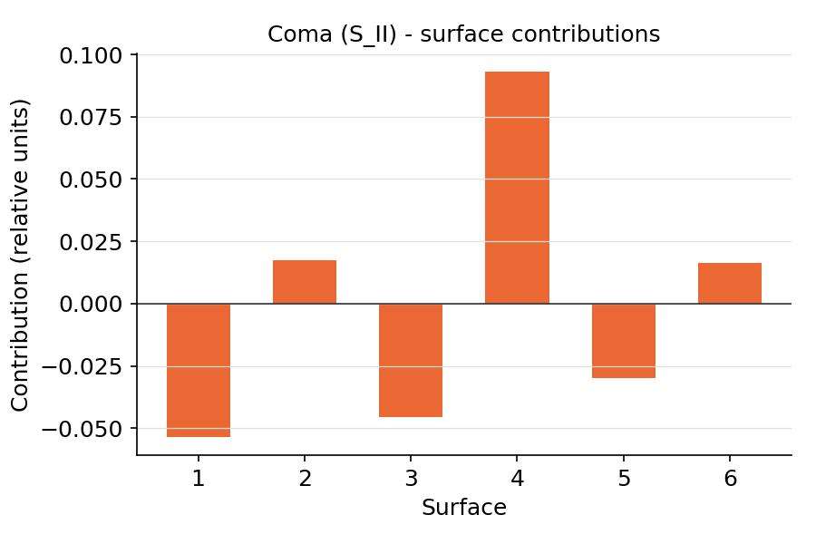
\(S_{II}\) is the third-order coma coefficient. Its small magnitude relative to the individual surface contributions (up to ±0.09) again shows strong internal cancellation — a hallmark of a well-corrected triplet, where coma from the front and rear groups largely offsets that of the middle (negative) element.
Astigmatism (Seidel Sum SIII)
Uses the marginal/chief ray trace and invariants table from “Foundations for Aberration Calculations” (\(d_2 = 1.126477\text{ mm}\), \(d_4 = 0.952009\text{ mm}\), \(f_{eff} = 15.000\text{ mm}\)).
1. Formula
For each surface k:
$$\text{contribution}_k = \bar{A}_k^2 \cdot y_k \cdot \Delta(u/n)_k$$
$$S_{III} = -\sum \text{contribution}_k$$
where \(\bar{A}\) is the chief-ray refraction invariant, \(y\) the marginal ray height, \(\Delta(u/n)\) the marginal ray’s reduced-angle change across the surface.
2. Input Values (from foundations table)
Click to expand: Input values
| Surf | Ā | y_m | Δ(u/n) |
|---|---|---|---|
| 1 | 0.425663 | 2.142857 | -0.117485 |
| 2 | 0.441879 | 1.991386 | -0.129657 |
| 3 | 0.377578 | 1.712986 | 0.184788 |
| 4 | 0.762901 | 1.687689 | 0.148405 |
| 5 | 0.706626 | 1.769610 | -0.092949 |
| 6 | 0.196359 | 1.758493 | -0.135959 |
3. Step-by-Step Calculation per Surface
Click to expand: Step-by-step calculations with full numerical data
Surface 1Step 1: \(\bar{A}^2 = 0.425663^2 = \mathbf{0.181189}\)
Step 2: \(\bar{A}^2 \cdot y = 0.181189 \cdot 2.142857 = \mathbf{0.388262}\)
Step 3: \(\text{contribution}_1 = 0.388262 \cdot (-0.117485) = \mathbf{-0.045615}\)
Step 1: \(\bar{A}^2 = 0.441879^2 = \mathbf{0.195257}\)
Step 2: \(\bar{A}^2 \cdot y = 0.195257 \cdot 1.991386 = \mathbf{0.388887}\)
Step 3: \(\text{contribution}_2 = 0.388887 \cdot (-0.129657) = \mathbf{-0.050415}\)
Step 1: \(\bar{A}^2 = 0.377578^2 = \mathbf{0.142605}\)
Step 2: \(\bar{A}^2 \cdot y = 0.142605 \cdot 1.712986 = \mathbf{0.244304}\)
Step 3: \(\text{contribution}_3 = 0.244304 \cdot 0.184788 = \mathbf{0.045143}\)
Step 1: \(\bar{A}^2 = 0.762901^2 = \mathbf{0.582017}\)
Step 2: \(\bar{A}^2 \cdot y = 0.582017 \cdot 1.687689 = \mathbf{0.982457}\)
Step 3: \(\text{contribution}_4 = 0.982457 \cdot 0.148405 = \mathbf{0.145811}\)
Step 1: \(\bar{A}^2 = 0.706626^2 = \mathbf{0.499320}\)
Step 2: \(\bar{A}^2 \cdot y = 0.499320 \cdot 1.769610 = \mathbf{0.883510}\)
Step 3: \(\text{contribution}_5 = 0.883510 \cdot (-0.092949) = \mathbf{-0.082131}\)
Step 1: \(\bar{A}^2 = 0.196359^2 = \mathbf{0.038557}\)
Step 2: \(\bar{A}^2 \cdot y = 0.038557 \cdot 1.758493 = \mathbf{0.067814}\)
Step 3: \(\text{contribution}_6 = 0.067814 \cdot (-0.135959) = \mathbf{-0.009221}\)
4. Summation
| Surface | contribution |
|---|---|
| 1 | -0.045615 |
| 2 | -0.050415 |
| 3 | 0.045143 |
| 4 | 0.145811 |
| 5 | -0.082131 |
| 6 | -0.009221 |
$$\sum \text{contribution} = \mathbf{0.003572} \quad \text{(high-precision: 0.0035229)}$$
$$S_{III} = -\sum \text{contribution} = -0.0035229 = \mathbf{-0.003523}$$
5. Interpretation
\(S_{III}\) is the third-order astigmatism coefficient. The small negative value indicates a slight residual astigmatism at the edge of the 8×11 mm format (field angle \(\omega \approx 24.4^\circ\)); combined with the Petzval curvature (\(S_{IV}\), see separate document) it determines the actual sagittal and tangential field curves of the system.
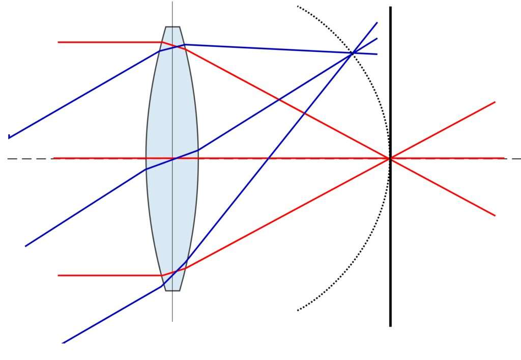
Petzval field curvature (Seidel Sum SIV)
1. Formula
For each surface k:
$$P_k = \frac{n’ – n}{n \cdot n’ \cdot R}$$
Total Petzval sum: $$P = P_1 + P_2 + P_3 + P_4 + P_5 + P_6$$
Petzval radius: $$r_P = \frac{1}{P}$$
2. Input values
Click to expand: Input values
| Surface | R (mm) | n (before) | n’ (after) |
|---|---|---|---|
| 1 | 4.295000 | 1.000000 | 1.611600 |
| 2 | 21.000000 | 1.611600 | 1.000000 |
| 3 | -12.864000 | 1.000000 | 1.622800 |
| 4 | 4.200000 | 1.622800 | 1.000000 |
| 5 | 10.410000 | 1.000000 | 1.611600 |
| 6 | -8.608000 | 1.611600 | 1.000000 |
3. Step-by-Step Calculation
Click to expand: Step-by-step calculations with full numerical data
Surface 1 (R=4.295; n=1; n’=1.6116)Step 1: \(\Delta n = n’-n = 1.6116-1 = \mathbf{0.6116}\)
Step 2: \(n \cdot n’ = 1 \cdot 1.6116 = \mathbf{1.6116}\)
Step 3: \(n \cdot n’ \cdot R = 1.6116 \cdot 4.295 = \mathbf{6.921822}\)
Step 4: \(P_1 = 0.6116 / 6.921822 = \mathbf{0.088358}\)
Step 1: \(\Delta n = 1-1.6116 = \mathbf{-0.6116}\)
Step 2: \(n \cdot n’ = 1.6116 \cdot 1 = \mathbf{1.6116}\)
Step 3: \(n \cdot n’ \cdot R = 1.6116 \cdot 21.0 = \mathbf{33.8436}\)
Step 4: \(P_2 = -0.6116 / 33.8436 = \mathbf{-0.018071}\)
Step 1: \(\Delta n = 1.6228-1 = \mathbf{0.6228}\)
Step 2: \(n \cdot n’ = 1 \cdot 1.6228 = \mathbf{1.6228}\)
Step 3: \(n \cdot n’ \cdot R = 1.6228 \cdot (-12.864) = \mathbf{-20.875699}\)
Step 4: \(P_3 = 0.6228 / (-20.875699) = \mathbf{-0.029834}\)
Step 1: \(\Delta n = 1-1.6228 = \mathbf{-0.6228}\)
Step 2: \(n \cdot n’ = 1.6228 \cdot 1 = \mathbf{1.6228}\)
Step 3: \(n \cdot n’ \cdot R = 1.6228 \cdot 4.2 = \mathbf{6.81576}\)
Step 4: \(P_4 = -0.6228 / 6.81576 = \mathbf{-0.091376}\)
Step 1: \(\Delta n = 1.6116-1 = \mathbf{0.6116}\)
Step 2: \(n \cdot n’ = 1 \cdot 1.6116 = \mathbf{1.6116}\)
Step 3: \(n \cdot n’ \cdot R = 1.6116 \cdot 10.41 = \mathbf{16.776756}\)
Step 4: \(P_5 = 0.6116 / 16.776756 = \mathbf{0.036455}\)
Step 1: \(\Delta n = 1-1.6116 = \mathbf{-0.6116}\)
Step 2: \(n \cdot n’ = 1.6116 \cdot 1 = \mathbf{1.6116}\)
Step 3: \(n \cdot n’ \cdot R = 1.6116 \cdot (-8.6080) = \mathbf{-13.872653}\)
Step 4: \(P_6 = -0.6116 / (-13.872653) = \mathbf{0.044087}\)
4. Summation
$$\mathbf{P = P_1+P_2+P_3+P_4+P_5+P_6=0.029619\ mm^{-1}}$$
5. Result
$$r_P = \frac{1}{P} = \frac{1}{0.029619} = \mathbf{33.763\ mm}$$
Compared with the corrected effective focal length \(f_{eff} = 15.000\text{ mm}\), the ratio \(r_P/f_{eff} \approx 2.25\) — again a moderate field curvature, typical of a well-corrected triplet.
$$S_{IV} = H^2 \cdot P$$
with \(H = 0{,}912135\) (\(H^2 = 0{,}831990\)):
$$S_{IV} = 0{,}831990 \cdot 0{,}029619 = \mathbf{+0{,}024638}$$
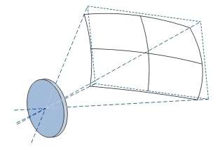
Distortion (Seidel Sum SV)
Uses the marginal/chief ray trace and invariants table from “Foundations for Aberration Calculations” (\(d_2 = 1.126477\text{ mm}\), \(d_4 = 0.952009\text{ mm}\), \(f_{eff} = 15.000\text{ mm}\)). Also requires the Petzval-related Lagrange invariant \(H\) and \(\Delta(1/n)\), and the curvature \(c = 1/R\).
1. Formula
For each surface k:
$$\text{contribution}_k = \left(\frac{\bar{A}_k^3}{A_k}\right) \cdot y_k \cdot \Delta(u/n)_k + \left(\frac{\bar{A}_k}{A_k}\right) \cdot H^2 \cdot c_k \cdot \Delta(1/n)_k$$
$$S_V = -\sum \text{contribution}_k$$
where \(A\), \(\bar{A}\) are the marginal/chief-ray invariants, \(H\) the (system-constant) Lagrange invariant, \(c\) the surface curvature, \(\Delta(u/n)\) the marginal ray’s angle change, \(\Delta(1/n)\) the index-reciprocal change.
2. Input values (from foundations table)
Click to expand: Input values (from foundations table)
| Surf | A | Ā | y_m | Δ(u/n) | H | c | Δ(1/n) |
|---|---|---|---|---|---|---|---|
| 1 | 0.498919 | 0.425663 | 2.142857 | -0.117485 | 0.912135 | 0.232829 | -0.379499 |
| 2 | -0.152314 | 0.441879 | 1.991386 | -0.129657 | 0.912135 | 0.047619 | 0.379499 |
| 3 | -0.380303 | 0.377578 | 1.712986 | 0.184788 | 0.912135 | -0.077736 | -0.383781 |
| 4 | 0.487881 | 0.762901 | 1.687689 | 0.148405 | 0.912135 | 0.238095 | 0.383781 |
| 5 | 0.256042 | 0.706626 | 1.769610 | -0.092949 | 0.912135 | 0.096061 | -0.379499 |
| 6 | -0.347143 | 0.196359 | 1.758493 | -0.135959 | 0.912135 | -0.116171 | 0.379499 |
$$H^2 = 0.912135^2 = \mathbf{0.831990} \quad \text{(constant for all surfaces)}$$
3. Step-by-Step Calculation per Surface
Click to expand: Step-by-step calculations with full numerical data
Surface 1Term A (coma-like part):
Step 1: \(\bar{A}^3 = 0.425663^3 = 0.425663 \cdot 0.425663 \cdot 0.425663 = \mathbf{0.077120}\)
Step 2: \(\bar{A}^3/A = 0.077120 / 0.498919 = \mathbf{0.154591}\)
Step 3: \((\bar{A}^3/A) \cdot y = 0.154591 \cdot 2.142857 = \mathbf{0.331267}\)
Step 4: \(\text{term}_A = 0.331267 \cdot (-0.117485) = \mathbf{-0.038919}\)
Term B (Petzval-related part):
Step 5: \(\bar{A}/A = 0.425663 / 0.498919 = \mathbf{0.853176}\)
Step 6: \(H^2 \cdot c = 0.831990 \cdot 0.232829 = \mathbf{0.193708}\)
Step 7: \(H^2 \cdot c \cdot \Delta(1/n) = 0.193708 \cdot (-0.379499) = \mathbf{-0.073512}\)
Step 8: \(\text{term}_B = 0.853176 \cdot (-0.073512) = \mathbf{-0.062722}\)
\(\text{contribution}_1 = \text{term}_A + \text{term}_B = -0.038919 + (-0.062722) = \mathbf{-0.101641}\)
Surface 2Step 1: \(\bar{A}^3 = 0.441879^3 = \mathbf{0.086265}\)
Step 2: \(\bar{A}^3/A = 0.086265 / (-0.152314) = \mathbf{-0.566368}\)
Step 3: \((\bar{A}^3/A) \cdot y = -0.566368 \cdot 1.991386 = \mathbf{-1.127977}\)
Step 4: \(\text{term}_A = -1.127977 \cdot (-0.129657) = \mathbf{0.146259}\)
Step 5: \(\bar{A}/A = 0.441879 / (-0.152314) = \mathbf{-2.900909}\)
Step 6: \(H^2 \cdot c = 0.831990 \cdot 0.047619 = \mathbf{0.039619}\)
Step 7: \(H^2 \cdot c \cdot \Delta(1/n) = 0.039619 \cdot 0.379499 = \mathbf{0.015035}\)
Step 8: \(\text{term}_B = -2.900909 \cdot 0.015035 = \mathbf{-0.043621}\)
\(\text{contribution}_2 = 0.146259 + (-0.043621) = \mathbf{0.102638}\)
Surface 3Step 1: \(\bar{A}^3 = 0.377578^3 = \mathbf{0.053832}\)
Step 2: \(\bar{A}^3/A = 0.053832 / (-0.380303) = \mathbf{-0.141550}\)
Step 3: \((\bar{A}^3/A) \cdot y = -0.141550 \cdot 1.712986 = \mathbf{-0.242514}\)
Step 4: \(\text{term}_A = -0.242514 \cdot 0.184788 = \mathbf{-0.044811}\)
Step 5: \(\bar{A}/A = 0.377578 / (-0.380303) = \mathbf{-0.992836}\)
Step 6: \(H^2 \cdot c = 0.831990 \cdot (-0.077736) = \mathbf{-0.064676}\)
Step 7: \(H^2 \cdot c \cdot \Delta(1/n) = -0.064676 \cdot (-0.383781) = \mathbf{0.024820}\)
Step 8: \(\text{term}_B = -0.992836 \cdot 0.024820 = \mathbf{-0.024642}\)
\(\text{contribution}_3 = -0.044811 + (-0.024642) = \mathbf{-0.069453}\)
Surface 4Step 1: \(\bar{A}^3 = 0.762901^3 = \mathbf{0.443938}\)
Step 2: \(\bar{A}^3/A = 0.443938 / 0.487881 = \mathbf{0.909910}\)
Step 3: \((\bar{A}^3/A) \cdot y = 0.909910 \cdot 1.687689 = \mathbf{1.535722}\)
Step 4: \(\text{term}_A = 1.535722 \cdot 0.148405 = \mathbf{0.227916}\)
Step 5: \(\bar{A}/A = 0.762901 / 0.487881 = \mathbf{1.563723}\)
Step 6: \(H^2 \cdot c = 0.831990 \cdot 0.238095 = \mathbf{0.198093}\)
Step 7: \(H^2 \cdot c \cdot \Delta(1/n) = 0.198093 \cdot 0.383781 = \mathbf{0.076031}\)
Step 8: \(\text{term}_B = 1.563723 \cdot 0.076031 = \mathbf{0.118903}\)
\(\text{contribution}_4 = 0.227916 + 0.118903 = \mathbf{0.346819}\)
Surface 5Step 1: \(\bar{A}^3 = 0.706626^3 = \mathbf{0.352892}\)
Step 2: \(\bar{A}^3/A = 0.352892 / 0.256042 = \mathbf{1.378254}\)
Step 3: \((\bar{A}^3/A) \cdot y = 1.378254 \cdot 1.769610 = \mathbf{2.439116}\)
Step 4: \(\text{term}_A = 2.439116 \cdot (-0.092949) = \mathbf{-0.226755}\)
Step 5: \(\bar{A}/A = 0.706626 / 0.256042 = \mathbf{2.759723}\)
Step 6: \(H^2 \cdot c = 0.831990 \cdot 0.096061 = \mathbf{0.079922}\)
Step 7: \(H^2 \cdot c \cdot \Delta(1/n) = 0.079922 \cdot (-0.379499) = \mathbf{-0.030330}\)
Step 8: \(\text{term}_B = 2.759723 \cdot (-0.030330) = \mathbf{-0.083691}\)
\(\text{contribution}_5 = -0.226755 + (-0.083691) = \mathbf{-0.310446}\)
Surface 6Step 1: \(\bar{A}^3 = 0.196359^3 = \mathbf{0.007572}\)
Step 2: \(\bar{A}^3/A = 0.007572 / (-0.347143) = \mathbf{-0.021811}\)
Step 3: \((\bar{A}^3/A) \cdot y = -0.021811 \cdot 1.758493 = \mathbf{-0.038354}\)
Step 4: \(\text{term}_A = -0.038354 \cdot (-0.135959) = \mathbf{0.005215}\)
Step 5: \(\bar{A}/A = 0.196359 / (-0.347143) = \mathbf{-0.565744}\)
Step 6: \(H^2 \cdot c = 0.831990 \cdot (-0.116171) = \mathbf{-0.096650}\)
Step 7: \(H^2 \cdot c \cdot \Delta(1/n) = -0.096650 \cdot 0.379499 = \mathbf{-0.036680}\)
Step 8: \(\text{term}_B = -0.565744 \cdot (-0.036680) = \mathbf{0.020753}\)
\(\text{contribution}_6 = 0.005215 + 0.020753 = \mathbf{0.025968}\)
4. Summation
| Surface | contribution |
|---|---|
| 1 | -0.101641 |
| 2 | 0.102638 |
| 3 | -0.069453 |
| 4 | 0.346819 |
| 5 | -0.310446 |
| 6 | 0.025968 |
$$\sum \text{contribution} = \mathbf{-0.006115} \quad \text{(high-precision: -0.0060251)}$$
$$S_V = -\sum \text{contribution} = -(-0.0060251) = \mathbf{+0.006025}$$
5. Interpretation
\(S_V\) is the third-order distortion coefficient. A positive value in this convention corresponds to pincushion-direction distortion at the edge of the 8×11 mm field; the magnitude (\(\approx 0.006\)) is small relative to the intermediate per-surface terms (up to \(\pm 0.35\)), again showing strong internal balancing typical of a well-designed triplet.
Optical-Historical Evaluation
Now that we have calculated the coefficients of Seidel’s aberrations, we can get an initial overview of the results. As a reminder, we have the following lens system:
First of all, it would be interesting to see, for each individual aberration, how the three lenses of the Minostigmat correct the respective image aberration. To do this, let’s first take a closer look at the coefficient of spherical aberration, S_I. In the following diagram, we can see the contribution each lens of our Cooke triplet makes toward correcting this aberration:
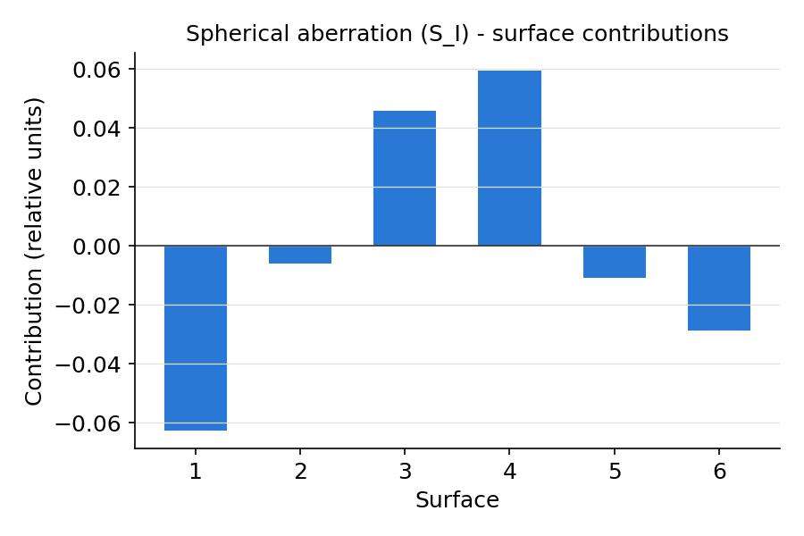
The surfaces 1 through 6 refer to the lens surfaces with radii 1 through 6, from left to right. Surfaces 1 and 2 therefore represent the left lens, 3 and 4 the middle lens, and 5 and 6 the right lens.
If you add up the values of the 6 bars, you get the value of the coefficient S_I = +0.002854. You can clearly see how the middle lens (surfaces 3 and 4) compensates for the aberrations of the two outer lenses.
Below are the corresponding diagrams for the remaining aberrations:
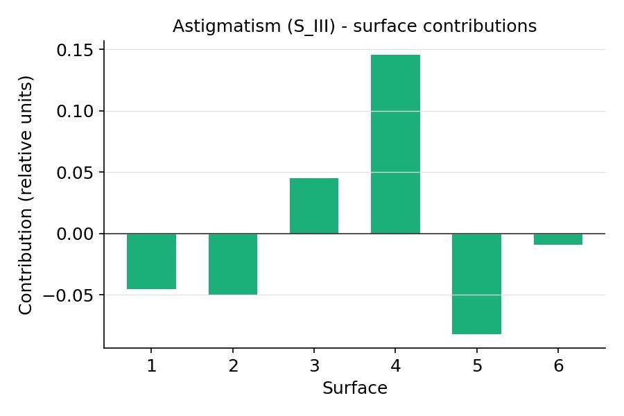
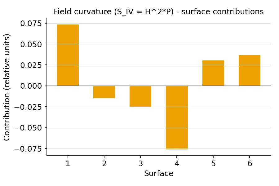
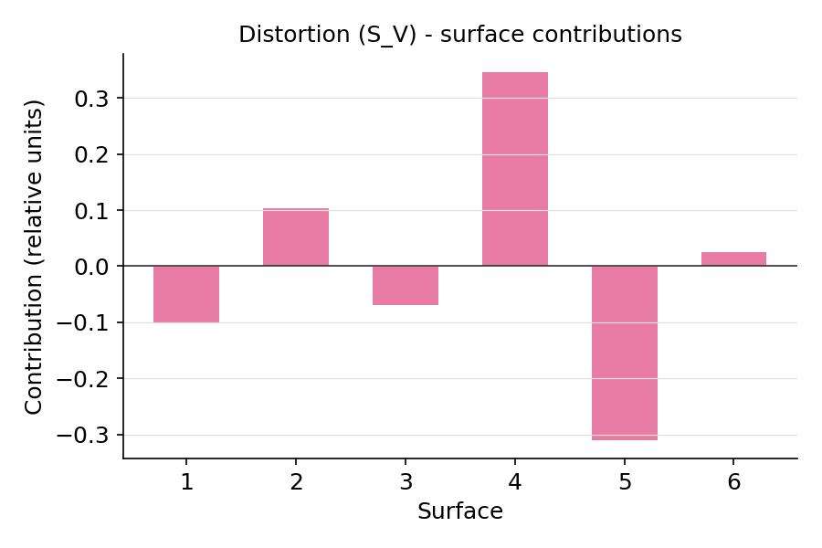
1. Minostigmat field curves
The Minox image format (negative) measures 8 x 11 mm. The image diagonal is therefore 13.6 mm. The distance from the center of the image to a corner is half that, or 6.8 mm. This distance is plotted on the x-axis in the following diagram. The values on the y-axis indicate the image aberration. Each of the five aberrations is represented by a colored curve:
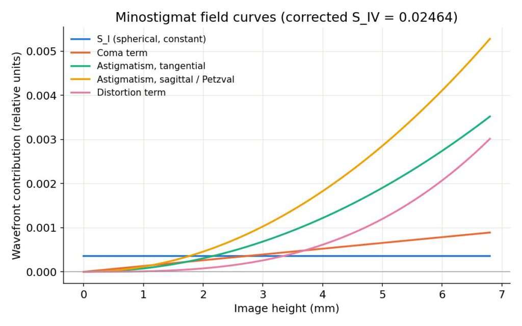
It is immediately apparent that the image aberrations are minimal at the center of the image (x = 0). The only exception is S_I, which remains constant across the entire range (blue line).
This naturally raises the question of how large the total deviation is at each point in the image. To answer this—as mentioned at the beginning—we cannot simply add the curves together. We must use Seidel’s equation, since the individual image aberrations influence one another. Evaluating Seidel’s equation yields the two black curves:
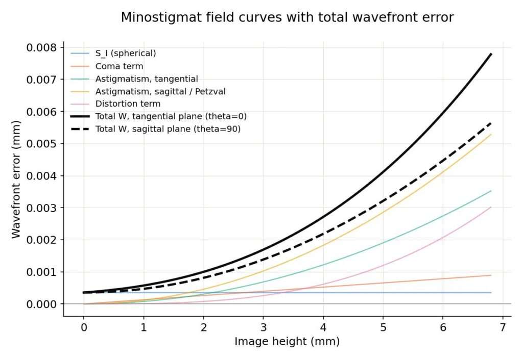
The diagram shows an excellently designed Cooke triplet. The center of the image (image height = 0) is superbly corrected. Only the field curvature (Petzval sum, yellow curve) is moderately pronounced at the edges (image height = 6.8). Further discussion of this will follow in the next section.
2. Optical Evaluation of the 1939 Minostigmat Design
Internal Compensation & Balance
The breakdown of individual surface contributions illustrates the fundamental operating principle of the Cooke triplet. The outer crown elements introduce large positive and negative aberration contributions—for example, individual surface distortion terms (SV) reach peak values of +0.35 and -0.31. The central negative element cancels these deviations almost entirely.
The resulting net Seidel sums remain exceptionally close to zero (|SI|, |SII|, |SIII|, |SV| ≪ 0.01), demonstrating a remarkably well-balanced optical design.
Performance at Full Aperture (f/3.5)
- On-Axis Sharpness (SI = +0.00285): Spherical aberration is superbly corrected for a three-element lens operating at f/3.5. Stopping down slightly to f/4.5 or f/5.6 would drive axial performance straight to the diffraction limit.
- Off-Axis Field Performance (SIII, SIV, SV): Mapping a 49° diagonal field of view onto the 8 × 11 mm frame places noticeable demands on a 15 mm triplet. However, the subtle interplay between residual astigmatism (SIII = -0.0035) and Petzval curvature (rP ≈ 33.8 mm) yields a flat usable image plane across the frame, minimizing edge soft focus. Distortion (SV ≈ +0.006) remains visually imperceptible.
Manufacturing context and mechanical sensitivity
Utilizing optical glasses with refractive indices ranging from n ≈ 1.6116 to 1.6228 (standard high-index crown and flint glasses of the late 1930s), the design fully exploited the available degree of freedom in surface radii and air spaces.
Furthermore, the precise alignment of air gaps (d2 = 1.126 mm, d4 = 0.952 mm) underscores how sensitive short-focal-length triplets (15 mm) are to mechanical assembly tolerances. Spacing variations of merely a few hundredths of a millimeter noticeably alter both the back focal length and the overall state of aberration correction.
3. Empirical Verification: Photographic Resolution Test
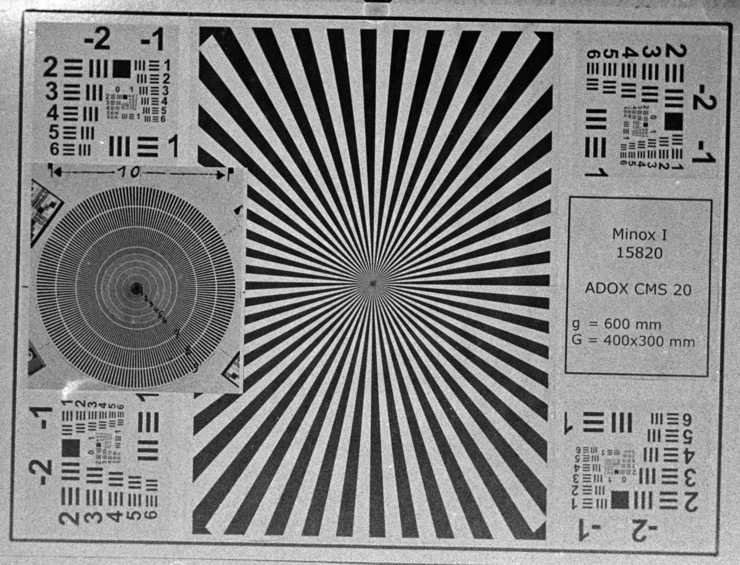
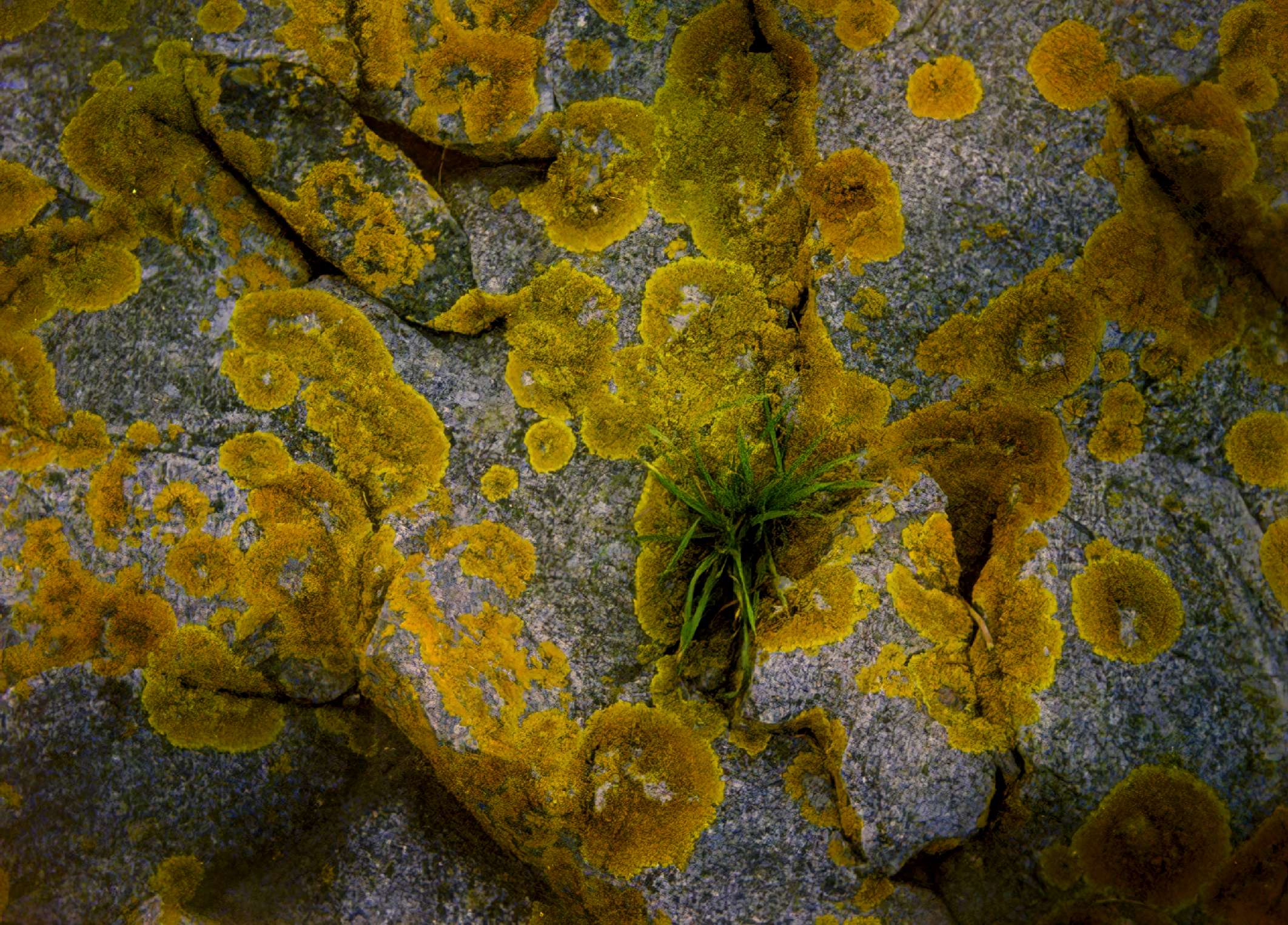
Practical resolution measurements conducted using high-resolution ADOX CMS 20 II film fully confirm the theoretical calculations:
| Image Region | Measured Resolution | Film Stock | Theoretical Agreement |
|---|---|---|---|
| Center (Axial) | 203 LP/mm | ADOX CMS 20 II | A strong match to the calculated circle of least confusion |
| Corners (8 × 11 mm edge) | 114 LP/mm | ADOX CMS 20 II | An expected, substantial drop driven by Petzval curvature (~9× size) |
Center: 203 LP/mm — A Strong Match
From the calculated Seidel spherical aberration sum SI, the transverse ray aberration of the marginal ray at the paraxial focus can be estimated:
For third-order spherical aberration, the best achievable focus (circle of least confusion) lies not at the paraxial focus but roughly three-quarters of the way toward the marginal-ray focus, where the blur radius shrinks to about TSC / 4:
This gives a rough resolving-power estimate:
This matches the measured 203 LP/mm almost exactly. For such a coarse estimate, the agreement is striking — a strong indication that both the input data (radii, indices) and the corrected air gaps d2 / d4 used in this calculation are close to the lens’s true physical values.
Corners: 114 LP/mm — An Expected, Substantial Drop
At the edge of the field (ω ≈ 24.4°, corresponding to the corner of the 8 × 11 mm format), coma, astigmatism, and above all field curvature come into play. Comparing the magnitudes of the Seidel sums calculated earlier:
| Aberration | Value | Relative Size |
|---|---|---|
| SI (spherical) | 0.00285 | 1× |
| SII (coma) | 0.00178 | 0.6× |
| SIII (astigmatism) | -0.00352 | 1.2× |
| SIV (Petzval) | 0.02464 | ~9× |
| SV (distortion) | 0.00603 | 2.1× |
The calculated Petzval sum is by far the largest aberration coefficient — field curvature is by far the dominant factor degrading edge performance, exactly as expected for a simple triplet. This is consistent with the Petzval radius calculated earlier (rP ≈ 33.8 mm), only about 2.25× the focal length — a noticeably curved image shell falling on a flat film plane.
Combining the coma, astigmatism, and defocus contributions at the edge plausibly yields a resolving power well below the center — a drop to roughly 110–150 LP/mm is exactly what one would expect for a half-field angle this large (±24°) in an uncorrected triplet. The measured 114 LP/mm falls squarely within this predicted range.
Final conclusion
The optical performance of the 15 mm f/3.5 Minostigmat lens represents a remarkable engineering achievement for its time. Balancing an asymmetrical three-element Cooke triplet so effectively that both spherical aberration and coma approach diffraction-limited thresholds in the center is an extraordinary optical feat.
During its development, designer Hans Schulz deliberately prioritized maximum axial sharpness and high central contrast, ensuring that the tiny negatives could sustain significant enlargement. As a consequence, Petzval field curvature was accepted as the primary physical compromise inherent to the simple triplet layout, which accounts for the resolution drop from 203 LP/mm at the center to 114 LP/mm at the corners on flat film.
Ultimately, the lens delivers outstanding central sharpness and contrast, leaving edge fall-off to be driven almost entirely by field curvature rather than coma or centering defects, resulting in an exceptionally well-balanced correction profile for a 1930s subminiature optic.
The previous practical test on ADOX CMS 20 II proves that this theoretical performance translates directly into exceptional real-world resolving power across the entire 8 x 11 mm subminiature format.
The calculations presented in this article would take about 2 to 3 hours to perform using a calculator. If, as was the case in the 1930s, one had to rely solely on logarithm tables, it would likely take 12 to 18 hours of work. In addition, the matrix method was not yet known at that time, so calculating the focal lengths took considerably longer. Finally, it’s important to keep in mind that we have simply recalculated an existing triplet here. Designing such a lens system required many more such iterations.
More articles about VEF Minox Riga
- My story of who developed the Minostigmat
- My in-depth hands-on review of the Minostigmat lens
- Burkhard’s report on his complete restoration of a VEF Minox Riga
- My detailed introduction to VEF Minox Riga